[Paper Review] ImageNet Classification with Deep Convolutional

Neural Networks (2012)

by- Shreyans Jain

Background

The AI community back in 2006 had this common belief, “a better algorithm would make better decisions, regardless of the data.” As we know nothing happens unanimously, there were critics regardingFei Fei Li who thought otherwise. According to her, “the best algorithm wouldn’t work well if the data it learned from didn’t reflect the real world”. So she set out to test out her hypothesis with a small team. The first instance of ImageNet was published as a research poster in 2009, it was a large scale image database. The philosophy behind ImageNet model is that we should for once shift our attendance from models to data. The dataset took two and a half years to complete. It consisted of 3.2 million labelled images, separated into 5,247 categories, sorted into 12 subtrees like “mammal,” “vehicle,” and “furniture.” It later evolved to 15 million images and 22,000 categories when this paper was published.

Motivation

Near human like recognition capabilities had been achieved on small datasets of similar images like the MNIST database. But objects in real settings exhibit variability and hence require a very large database. As I mentioned earlier for the first time, a one of a kind database was published that had millions of labeled images. An annual competition called the ImageNet Large-Scale Visual Recognition Challenge (ILSVRC) has been held which led the team of highly motivated researchers to finally pick up the challenge. The current models were also prohibitively large and expensive to train.

AlexNet

The model developed was named AlexNet by the authors. The complete details of developing it are:

Data Preprocessing:

The ImageNet contained images of variable resolutions which presents major problems.

Neural networks expect inputs to be of the same shape, hence require Using high res images may also present the problem of overfitting, reducing the complexity of data encourages the model to learn more generalised features. Eg a stone in a picture of a beach presents no significance but a high res image may force the network to also see it as a feature of a beach.

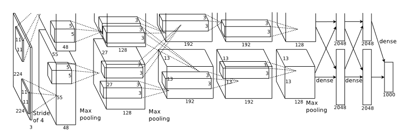
Architecture:

The nn consisted of 8 layers, 5 convolutional and 3 fully connected. This number was reached to ensure maximum accuracy and was observed that dropping even one of the fully connected layers presented a major decrease in accuracy.
Activation Function: ReLU (Rectified liner Unit- max(0,x) ) was used as the activation function between the layers. The usual activation functions are sigmoid and tanh(x). But they present the challenge of saturation in the neural network. ReLU also allowed for faster training as its less computationally expensive.

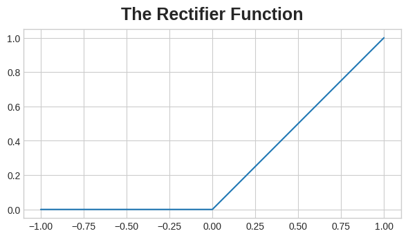
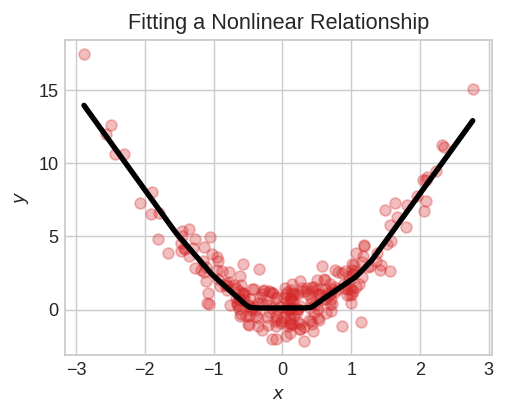
The heart of neural network in a way lies in the activation function as it enables it to learn something non-linear. “Two dense layers with nothing in between are no better than a single dense layer by itself. Dense layers by themselves can never move us out of the world of lines and planes. What we need is something nonlinear. What we need are activation functions.”
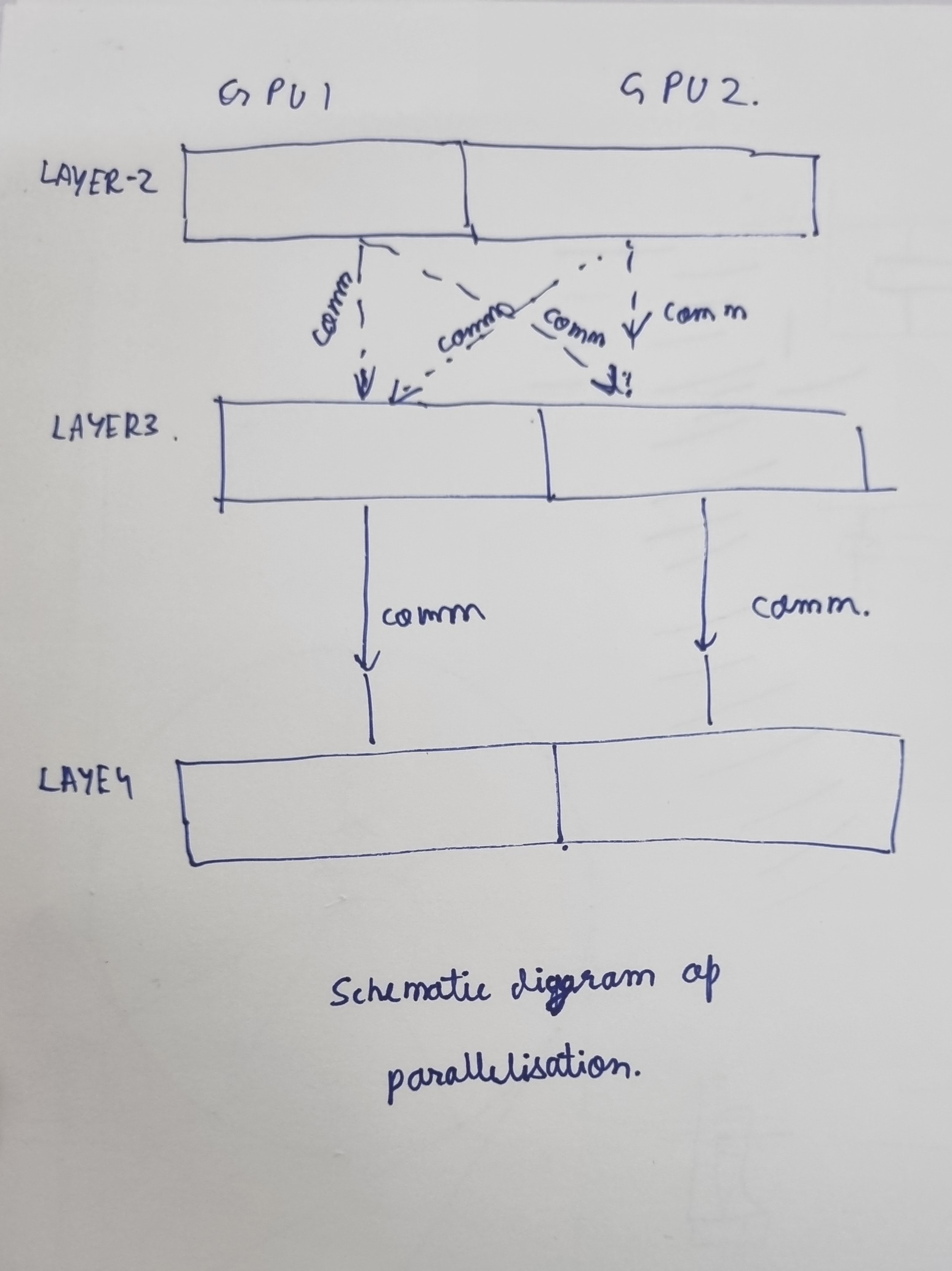
Parallelizing Training: The state of the art GPU was a GTX 580 3GB (Which was succeeded with a superior GTX 680 just two months after the release of the paper). The GPUs were connected in SLI which enabled to read and write to each others memory without going to the host machine. The layers are connected in a way that tries to minimize communication between the GPUs while still enabling effective training. A schematic simplified representation is shown in the image below.
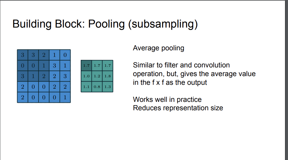
Pooling: Given below is how average pooling works here the stride=1 and neighborhood size=3, similarly Alexnet employed stride=2 and neighborhood size=3. Through hyperparameter tuning it was found that these particular values provided a performance boost. Additionally it was experimentally found that this helped prevent overfitting.
Local Response Normalization: Features that tend to produce activations of very different sizes can make for unstable training behavior. In shallow networks we often use scikit learns StandardScaler to bring the input on a similar scale so there is no bias due to magnitude of numeric values. Somewhat similar concept applies here, we normalize the responses in a certain neighborhood.

normalized_response = original_response / (k + alpha * sum(squared_responses)).

k is a constant hyperparameter to avoid division by zero and control the amplification factor.
alpha is a hyperparameter that determines the degree of normalization.
squared_responses represents the squared values of the responses within the local neighborhood window

This aids generalization and prevents overfitting. The purpose is to amplify the output of neurons that have relatively large activation. This practice has reduced nowadays and in fact, we have a special kind of layer that can do this, the batch normalization layer. A batch normalization layer looks at each batch as it comes in, first normalizing the batch with its own mean and standard deviation, and then also putting the data on a new scale with two trainable rescaling parameters. Batchnorm, in effect, performs a kind of coordinated rescaling of its inputs.

Reducing Overfitting

The network architecture consisted of 60 million parameters. Although the training set is large its insufficient to prevent overfitting. It was taken care of in the following to ways.

Data Augmentation

This refers to artificially increasing the size of the dataset. The stroke of genius here is that we can do so on free compute (time wise) the images are transformed on a cpu while the gpu is busy training the previous set of images . The data was augmented in two ways, the first was generating image translations and horizontal reflections. We do this by extracting random 224 × 224 patches (and their horizontal reflections) from the 256×256 images. The second is altering RGB values by PCA. To each image certain multiples of found pca components are added. This scheme works as an object lets say a chair is invariant to intensity of illumination or colour.

Dropout

Overfitting makes the model learn spurious patterns. Since these spurious patterns are so specific they are very easy to break if that particular neuron is deactivated. In dropout we randomly drop out some fraction of input units, this makes it very hard to overfit and more generalized patterns are learned as they are more prominent in every pass and are present even after dropout. Here dropout was kept at 50%. Although it does increase the number of iteration required.

Details of learning:

Stochastic gradient descent was used. The batch size of 128, momentum of 0.9 and weight decay =0.0005.

Momentum: Momentum is a technique that helps accelerate the convergence of the optimization process and overcome the local minima in the loss landscape. It simulates the behavior of a moving object with momentum. In the context of neural networks, it introduces a “velocity” term that influences the update of the model’s parameters.

velocity = momentum * velocity - learning_rate * gradient parameters = parameters + velocity

velocity represents the accumulated velocity from previous iterations.
momentum is a hyperparameter that determines the influence of the previous velocities on the current update.
learning_rate is the rate at which the model learns from the gradients.
gradient represents the gradient of the loss function with respect to the parameters.
parameters are the model’s weights and biases.

Decay is to prevent the model from relying on any single feature, so its a penalty added to the loss function. parameters = parameters - learning_rate * (gradient + weight_decay * parameters)

It penalizes larger weights more.

Also the weights instead of being random were initialised as follows, “We initialized the weights in each layer from a zero-mean Gaussian distribution with standard deviation 0.01. We initialized the neuron biases in the second, fourth, and fifth convolutional layers, as well as in the fully-connected hidden layers, with the constant 1. “ This was to accelerated learning by providing ReLU with positive inputs.

Results

Learning rate was kept constant and manually adjusted by seeing the validation error rate.

The network won the ILSCVRC-2010 with top-1 and top-5test set error rates of 37.5% and 17.0%5.

Future Scope

Use of unsupervised learning to find patterns in data could potentially help. Like setting weights based on it and then tuning it by supervised learning has the potential to increase the accuracy. Further doing this task on video sequences it can see how data evolves and can help in identifying features even better.